AdaptDiffuser: Misleading Results

2024-10-10

The paper AdaptDiffuser: Diffusion Models as Adaptive Self-evolving Planners is a research paper in offline RL accepted at ICML 2023. However, upon closer inspection, the presentation of the results raises several concerns that are worth highlighting. These issues, while potentially unintentional, could mislead readers into drawing conclusions that are not fully supported by the data.

Results Comparison: Missing the Full Picture

Let’s start by examining the results from the paper, specifically Table 2. It compares AdaptDiffuser’s performance to several baseline algorithms using the D4RL benchmarks. The results were calculated across three random seeds for AdaptDiffuser and the baselines, while Diffuser results are averaged over 150 seeds.

Dataset	Environment	BC	CQL	IQL	DT	TT	MOPO	MOReL	MBOP	Diffuser	AdaptDiffuser
Med-Expert	HalfCheetah	55.2	91.6	86.7	86.8	95.0	63.3	53.3	105.9	88.9 ± 0.3	89.6 ±0.8
Med-Expert	Hopper	52.5	105.4	91.5	107.6	110.0	23.7	108.7	55.1	103.3 ± 1.3	111.6 ±2.0
Med-Expert	Walker2d	107.5	108.8	109.6	108.1	101.9	44.6	95.6	70.2 ± 106.9	106.9	108.2 ±0.8
Medium	HalfCheetah	42.6	44.0	47.4	42.6	46.9	42.3	42.1	44.6	42.8 ± 0.3	44.2 ±0.6
Medium	Hopper	52.9	58.5	66.3	67.6	61.1	28.0	95.4	48.8	74.3 ± 1.4	96.6 ±2.7
Medium	Walker2d	75.3	72.5	78.3	74.0	79.0	17.8	77.8	41.0	79.6 ± 0.55	84.4 ±2.6
Med-Replay	HalfCheetah	36.6	45.5	44.2	36.6	41.9	53.1	40.2	42.3	37.7 ± 0.5	38.3 ±0.9
Med-Replay	Hopper	18.1	95.0	94.7	82.7	91.5	67.5	93.6	12.4	93.6 ± 0.4	92.2 ±1.5
Med-Replay	Walker2d	26.0	77.2	73.9	66.6	82.6	39.0	49.8	9.7	70.6 ± 1.6	84.7 ±3.1
Average		51.9	77.6	77.0	74.7	78.9	42.1	72.9	47.8	77.5	83.4

At first glance, the table suggests that AdaptDiffuser either matches or outperforms competing algorithms across most environments. However, the comparison methodology raises a few red flags. The use of only three seeds to evaluate AdaptDiffuser, especially given RL algorithms’ notorious variance, is insufficient to draw reliable conclusions. Diffuser, on the other hand, used 150 seeds—making the comparison far from apples-to-apples.

Why Seeds Matter: High Variance in RL Algorithms

Reinforcement learning algorithms are highly sensitive to initialization and hyperparameter choices. As a result, performance across different seeds can vary significantly. Averaging results over only three seeds doesn’t provide a sufficiently strong basis to claim superiority of an algorithm. This is why we typically see research papers using many more seeds to account for variance and improve reproducibility.

In fact, the use of standard error to report results is problematic in this context. Standard error gives an overly optimistic sense of precision because it doesn't capture the true spread of results. Instead, confidence intervals should be used. Unlike standard error, confidence intervals offer a more accurate reflection of the uncertainty in the performance estimates.

Confidence Intervals Show a Different Story

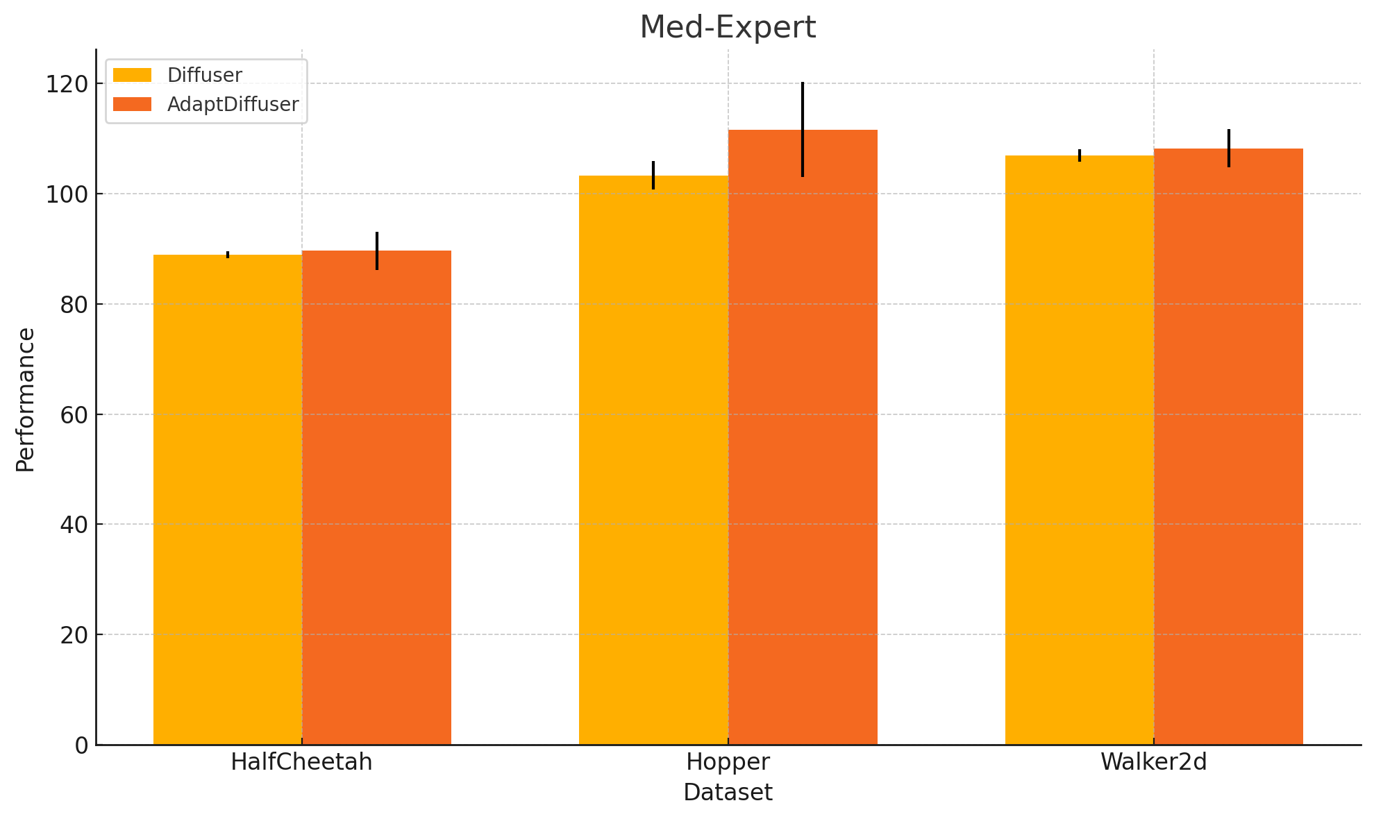
Let’s calculate and visualize the 95% confidence intervals for both Diffuser and AdaptDiffuser. Below, you can see how the confidence intervals of these two models overlap significantly, indicating that we cannot say with 95% confidence that one outperforms the other.

Code to calculate confidence intervals

import scipy.stats as stats
import numpy as np

data = {
    "Diffuser": [
        (88.9, 0.3),
        (103.3, 1.3),
        (106.9, 0.55),
        (42.8, 0.3),
        (74.3, 1.4),
        (79.6, 0.55),
        (37.7, 0.5),
        (93.6, 0.4),
        (70.6, 1.6)
    ],
    "AdaptDiffuser": [
        (89.6, 0.8),
        (111.6, 2.0),
        (108.2, 0.8),
        (44.2, 0.6),
        (96.6, 2.7),
        (84.4, 2.6),
        (38.3, 0.9),
        (92.2, 1.5),
        (84.7, 3.1)
    ]
}

n_diffuser = 150
n_adaptdiffuser = 3

confidence_level = 0.95
t_diffuser = stats.t.ppf((1 + confidence_level) / 2., n_diffuser - 1)
t_adaptdiffuser = stats.t.ppf((1 + confidence_level) / 2., n_adaptdiffuser - 1)

def confidence_interval(mean, std_err, t_value, n):
    margin_of_error = t_value * std_err
    lower_bound = mean - margin_of_error
    upper_bound = mean + margin_of_error
    return lower_bound, upper_bound

diffuser_ci = [confidence_interval(mean, std_err, t_diffuser, n_diffuser) for mean, std_err in data["Diffuser"]]
adaptdiffuser_ci = [confidence_interval(mean, std_err, t_adaptdiffuser, n_adaptdiffuser) for mean, std_err in data["AdaptDiffuser"]]

diffuser_ci, adaptdiffuser_ci

Code to plot the results

import matplotlib.pyplot as plt

# Data preparation
datasets = ['HalfCheetah', 'Hopper', 'Walker2d']
envs = ['Med-Expert', 'Medium', 'Med-Replay']

# Split confidence intervals into groups by environment
diffuser_ci_med_expert = diffuser_ci[:3]
adaptdiffuser_ci_med_expert = adaptdiffuser_ci[:3]

diffuser_ci_medium = diffuser_ci[3:6]
adaptdiffuser_ci_medium = adaptdiffuser_ci[3:6]

diffuser_ci_med_replay = diffuser_ci[6:]
adaptdiffuser_ci_med_replay = adaptdiffuser_ci[6:]

# Function to plot data
def plot_ci(data_diffuser, data_adaptdiffuser, title):
    x = np.arange(len(datasets))
    width = 0.35  

    fig, ax = plt.subplots()
    
    ax.bar(x - width/2, [(ci[0] + ci[1]) / 2 for ci in data_diffuser], width, 
           yerr=[(ci[1] - ci[0]) / 2 for ci in data_diffuser], label='Diffuser', capsize=5)
    ax.bar(x + width/2, [(ci[0] + ci[1]) / 2 for ci in data_adaptdiffuser], width, 
           yerr=[(ci[1] - ci[0]) / 2 for ci in data_adaptdiffuser], label='AdaptDiffuser', capsize=5)

    ax.set_xlabel('Dataset')
    ax.set_ylabel('Performance')
    ax.set_title(title)
    ax.set_xticks(x)
    ax.set_xticklabels(datasets)
    ax.legend()

    fig.tight_layout()

    plt.show()

plot_ci(diffuser_ci_med_expert, adaptdiffuser_ci_med_expert, 'Med-Expert')

plot_ci(diffuser_ci_medium, adaptdiffuser_ci_medium, 'Medium')

plot_ci(diffuser_ci_med_replay, adaptdiffuser_ci_med_replay, 'Med-Replay')

Med-Expert plot with confidence intervals

Expand to see plots for Medium and Med-Replay

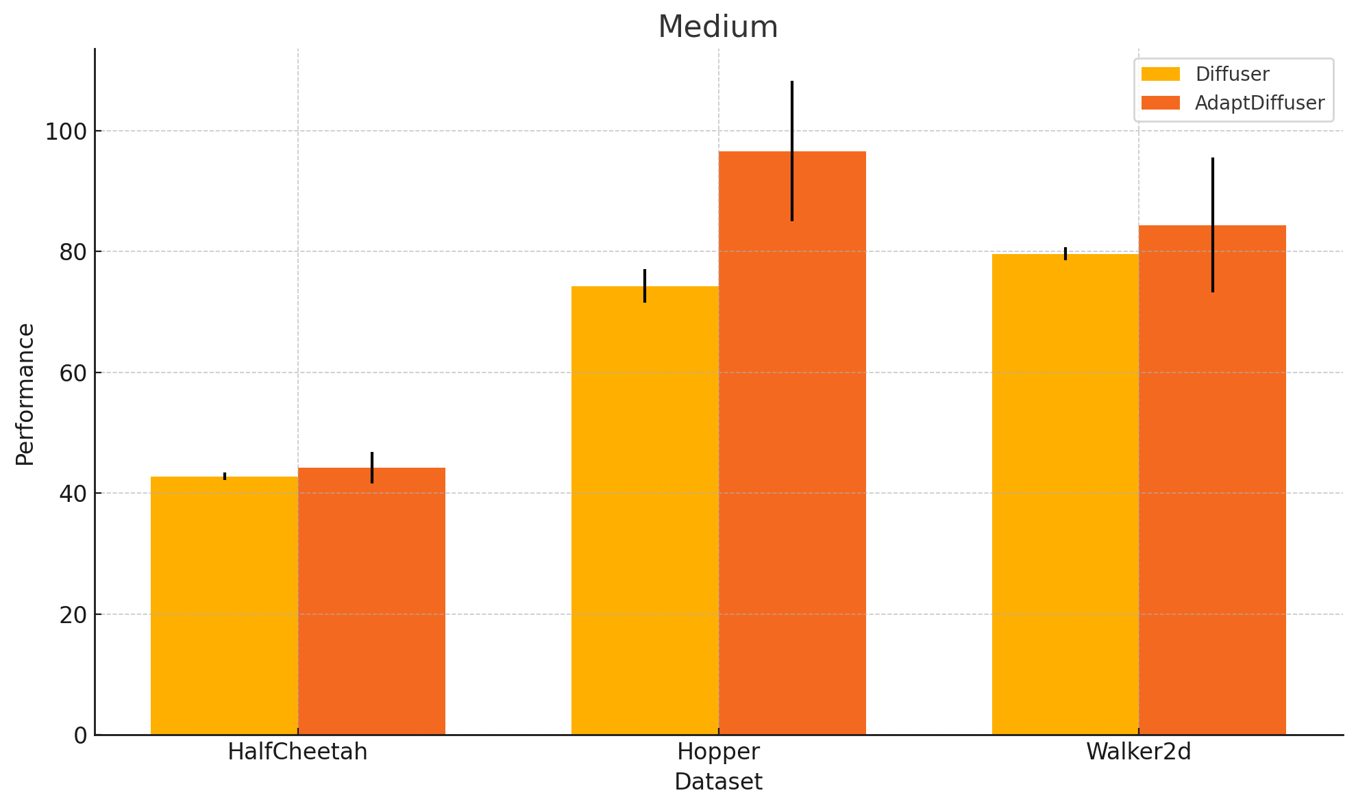
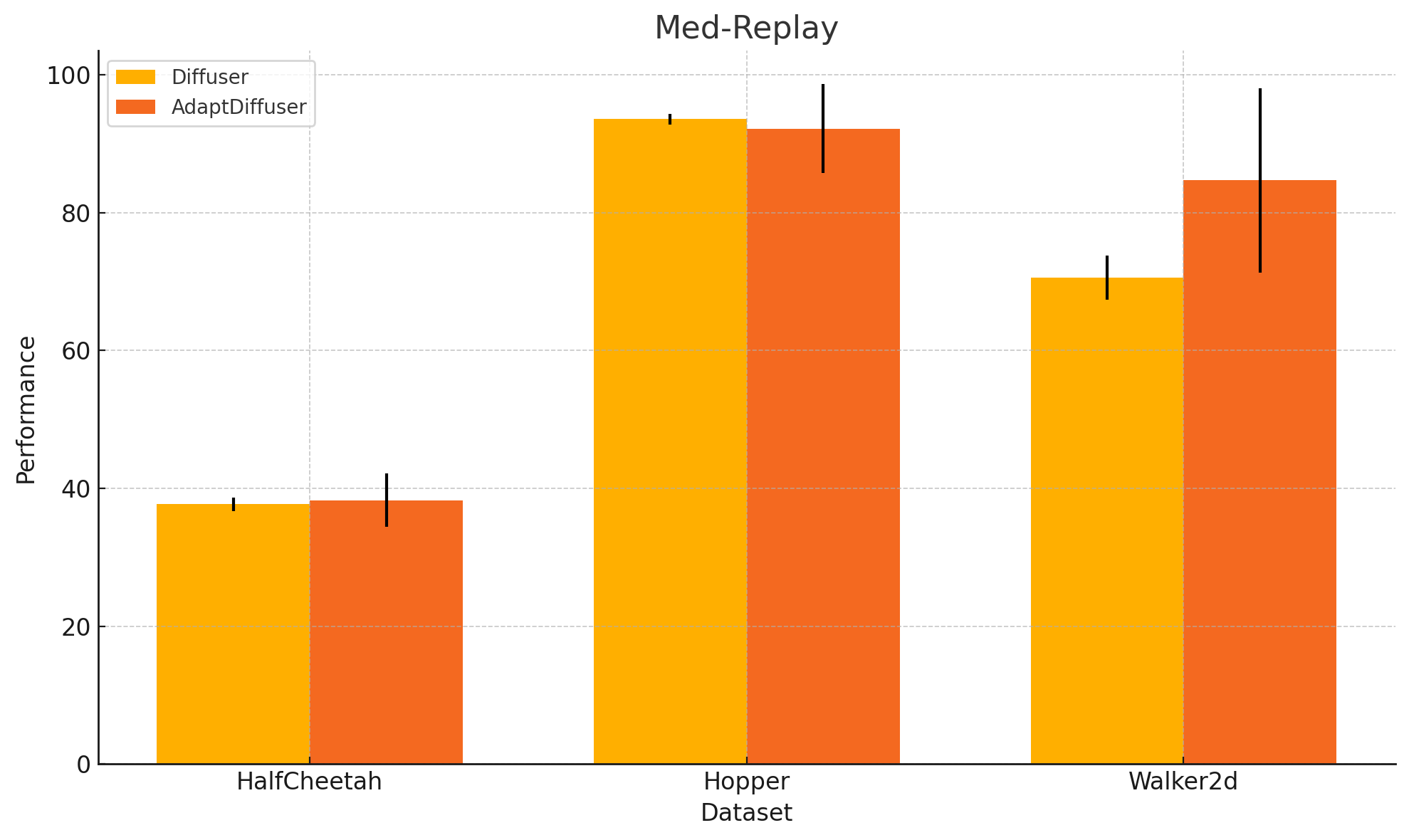
Medium plot with confidence intervals Med-Replay plot with confidence intervals

As we can see, the confidence intervals for Diffuser and AdaptDiffuser overlap across all environments. This means we cannot assert with confidence that AdaptDiffuser consistently outperforms Diffuser, despite the impression one might get from the standard error bars alone.

The Bigger Problem: Inflating Results in RL Research

This brings us to a broader issue in RL research: why are so many papers, including AdaptDiffuser, using only a small number of seeds and standard error to present their results? It leads to misleading conclusions, especially when confidence intervals would paint a more accurate picture.

A more robust experimental approach would involve:

Using more seeds to account for the high variance typical of RL algorithms.
Presenting confidence intervals rather than standard errors to give a clearer understanding of the algorithm's performance.

Conclusion: Questioning Research Rigor

The results presented in AdaptDiffuser, while intriguing, don’t hold up to closer scrutiny. The use of only three seeds and standard error creates a misleading narrative about the algorithm's superiority. This issue isn’t isolated to one paper. It reflects a broader trend in RL research, where high variance algorithms and limited experimental rigor can lead to misleading conclusions. I believe for the field to move forward meaningfully, we need to adopt higher standards for reproducibility and transparency.

Bonus: Comparing AdaptDiffuser with Baseline Algorithms

For a more complete picture, let's also compare AdaptDiffuser with baseline algorithms like BC, CQL, IQL, DT, TT, MOPO, MOReL, and MBOP. Although the paper did not provide the standard errors for these baselines, we can estimate them as 5% of their mean performance to approximate confidence intervals.

Here’s the code for calculating the estimated standard errors and confidence intervals for the baselines:

Expand to see code for baseline confidence intervals

import scipy.stats as stats
import numpy as np

# Performance data for baseline algorithms
other_methods_data = {
    "BC": [55.2, 52.5, 107.5, 42.6, 52.9, 75.3, 36.6, 18.1, 26.0],
    "CQL": [91.6, 105.4, 108.8, 44.0, 58.5, 72.5, 45.5, 95.0, 77.2],
    "IQL": [86.7, 91.5, 109.6, 47.4, 66.3, 78.3, 44.2, 94.7, 73.9],
    "DT": [86.8, 107.6, 108.1, 42.6, 67.6, 74.0, 36.6, 82.7, 66.6],
    "TT": [95.0, 110.0, 101.9, 46.9, 61.1, 79.0, 41.9, 91.5, 82.6],
    "MOPO": [63.3, 23.7, 44.6, 42.3, 28.0, 17.8, 53.1, 67.5, 39.0],
    "MOReL": [53.3, 108.7, 95.6, 42.1, 95.4, 77.8, 40.2, 93.6, 49.8],
    "MBOP": [105.9, 55.1, 70.2, 44.6, 48.8, 41.0, 42.3, 12.4, 9.7]
}

# Assume all baseline methods have n=3 and we estimate the standard error (SE) as 5% of the mean
n_others = 3
confidence_level = 0.95
t_other = stats.t.ppf((1 + confidence_level) / 2., n_others - 1)

def estimate_standard_error(mean):
    return mean * 0.05  # 5% of the mean

def confidence_interval(mean, std_err, t_value, n):
    margin_of_error = t_value * std_err
    lower_bound = mean - margin_of_error
    upper_bound = mean + margin_of_error
    return lower_bound, upper_bound

# Calculate confidence intervals for baseline algorithms
other_methods_ci = {}
for method, means in other_methods_data.items():
    ci = [confidence_interval(mean, estimate_standard_error(mean), t_other, n_others) for mean in means]
    other_methods_ci[method] = ci

other_methods_ci

Visualizing the Comparisons

Now, let’s visualize these comparisons, showing the confidence intervals for all the algorithms, including Diffuser and AdaptDiffuser. Below is a comparison for the Med-Expert environment:

Code

# Plotting code for all methods (including Diffuser and AdaptDiffuser) with confidence intervals
import numpy as np
import matplotlib.pyplot as plt

datasets = ['HalfCheetah', 'Hopper', 'Walker2d']
env_datasets = ['Med-Expert', 'Medium', 'Med-Replay']
methods_with_diffusers = ['BC', 'CQL', 'IQL', 'DT', 'TT', 'MOPO', 'MOReL', 'MBOP', 'Diffuser', 'AdaptDiffuser']

def plot_all_methods_ci_with_diffusers(ci_data, title):
    x = np.arange(len(datasets))  # the label locations
    width = 0.08  # adjust width for more bars
    fig, ax = plt.subplots(figsize=(12, 6))
    
    for i, method in enumerate(methods_with_diffusers):
        means = [(ci[0] + ci[1]) / 2 for ci in ci_data[method]]
        errors = [(ci[1] - ci[0]) / 2 for ci in ci_data[method]]
        ax.bar(x + i * width - (len(methods_with_diffusers) / 2) * width, means, width, 
               yerr=errors, label=method, capsize=5)
    
    ax.set_xlabel('Dataset')
    ax.set_ylabel('Performance')
    ax.set_title(title)
    ax.set_xticks(x)
    ax.set_xticklabels(datasets)
    ax.legend(loc='best', bbox_to_anchor=(1, 1))

    plt.tight_layout()
    plt.show()

plot_all_methods_ci_with_diffusers(other_methods_ci, 'Med-Expert')

All algorithms: Med-Expert

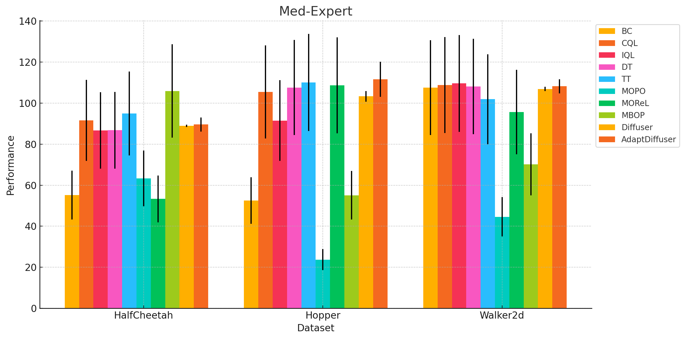
Expand to see results for Medium and Med-Replay

All algorithms: Medium All algorithms: Med-Replay

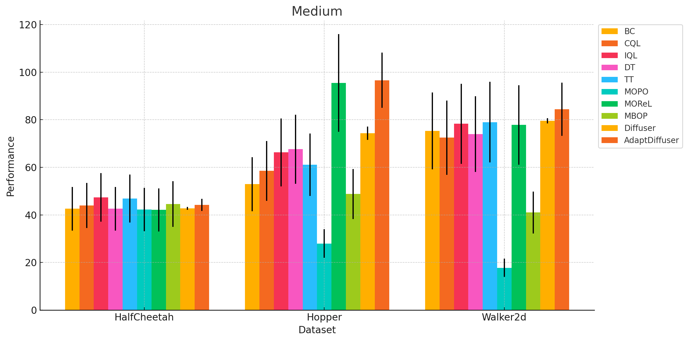
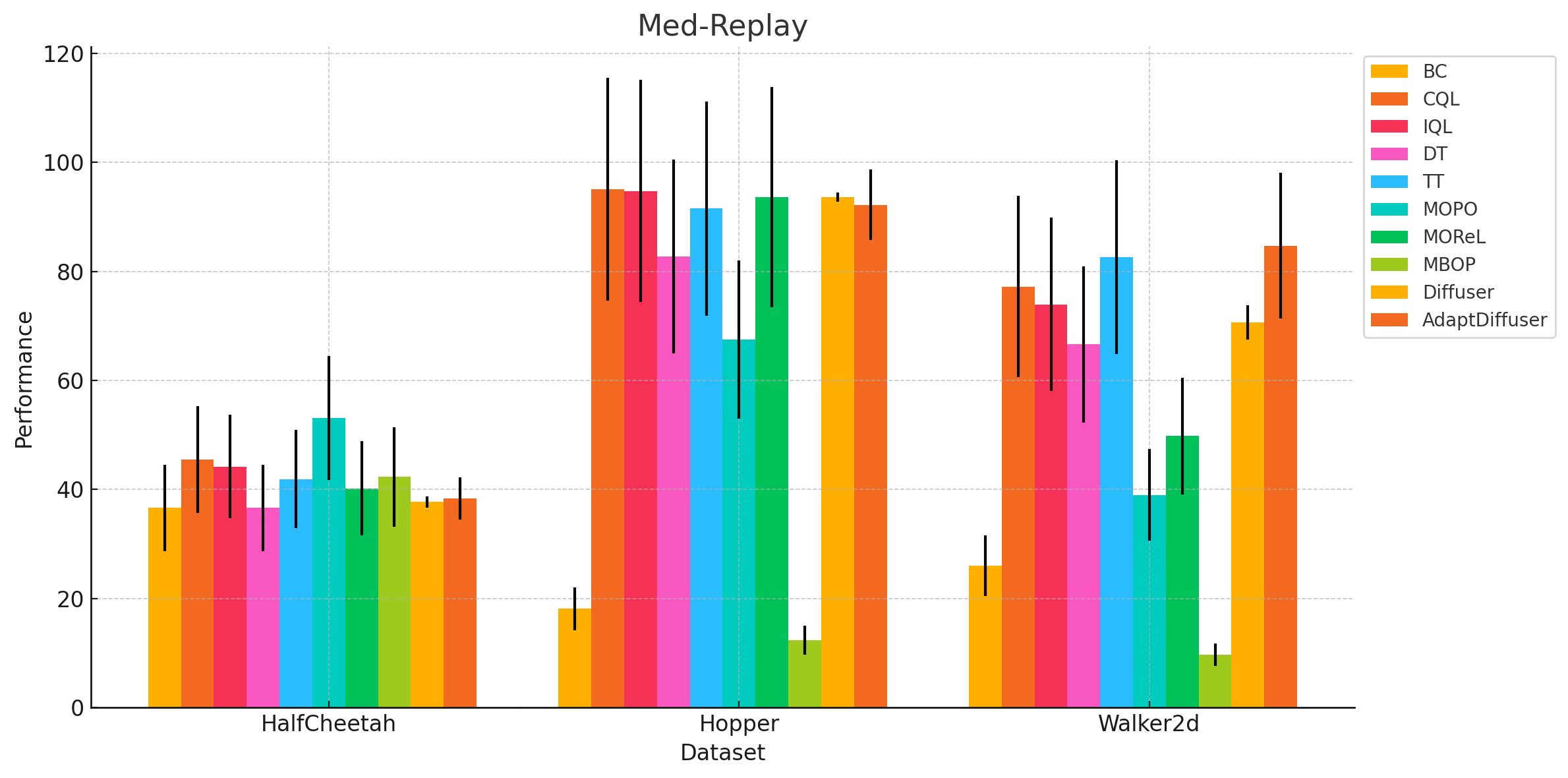
As we can see from the visualizations, the confidence intervals across the baseline algorithms overlap quite a bit with Diffuser and AdaptDiffuser. This suggests that we cannot definitively conclude that AdaptDiffuser outperforms other algorithms across all environments.